Real-world multi-scale analysis of colorectal cancer H&E¶

From H&E slides to tissue contexts, cell neighborhoods and patient-level analyses with ALHENA

This use case applies ALHENA to two public colorectal cancer cohorts and demonstrates how its tile embeddings, cell embeddings and cell annotations can be reused across tissue-level, spatial and patient-level analyses.

Each slide is encoded once. The resulting tile and cell representations, together with the cell annotations, are stored in scverse-compatible objects and reused throughout the workflow with Scanpy, SpatialData and Squidpy.

ALHENA is applied to both cohorts as provided, without cohort-specific fitting or calibration.

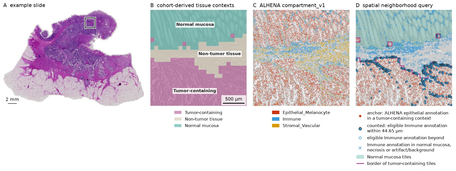
Overview of the workflow on one example slide. ALHENA tile embeddings are grouped into tissue contexts, cell embeddings receive cell type annotations, and the two scales are combined in a spatial neighborhood query. The outline in panel A marks the region enlarged in panels B to D. Image from BioImage Archive S-BIAD1407, CC BY 4.0.

All quantitative results use complete slides. Smaller regions from BRAF_094_CT_CBM_P1 are shown only to make the spatial outputs easier to inspect.

Code blocks show the analysis workflow. Displayed outputs are frozen results from the completed analysis.

Cohorts, ALHENA inputs and data from the original study¶

This example reuses two of the colorectal cancer cohorts described by Trahearn et al. (J Pathol, 2025), BRAF and MISSONI, together with their associated public data resources. H&E slides are available from BioImage Archive S-BIAD1407, while nucleus coordinates and the cell labels reported in the study are available from Mendeley Data 9z48yfzr63. Microsatellite instability (MSI) status is taken from the original publication.

ALHENA receives only the H&E slides and nucleus coordinates. The published cell labels and MSI status are not used to generate ALHENA embeddings or annotations: the cell labels are introduced only afterward to compare annotation systems, and MSI status is used only as the outcome for the patient-level classification analysis.

Role	Data
Inputs to ALHENA	H&E slides and nucleus coordinates
Data from the original study used downstream	Cell labels used to compare ALHENA annotations; MSI status used as the outcome for patient-level classification

The archive contains 229 primary-tumor slides. After technical quality control for file integrity and coordinate alignment, 212 slides from 209 patients remain for analysis. No slide is excluded based on its histological appearance.

The code uses alhena[spatial,wsi] and Squidpy 1.8.2 or later.

import numpy as np
import pandas as pd
import spatialdata as sd
import squidpy as sq

import alhena
from alhena import io, spatial

The retained slides are described by slide_manifest, one row per slide. n_tissue_tiles counts the 95 µm tiles of a slide that hold at least 25% tissue; ALHENA encodes those tiles.

slide_manifest.head()

	patient_id	cohort	n_tissue_tiles
slide_id
BRAF/004_AT_PD_P1	BRAF-004	BRAF	44749
BRAF/006_AA_CBM_P1	BRAF-006	BRAF	44702
BRAF/008_AN_PD_P1	BRAF-008	BRAF	52991
BRAF/009_AS_PD_P1	BRAF-009	BRAF	83879
BRAF/010_AM_PD_P1	BRAF-010	BRAF	46052

Encode each slide once with ALHENA¶

slide_inputs stores the image input, tissue-tile coordinates and nucleus-coordinate file for each slide. Each row stores the inputs for one slide.

slide_inputs.loc[
    ["BRAF/094_CT_CBM_P1"],
    ["image", "tissue_tiles", "nuclei"],
]

	image	tissue_tiles	nuclei
slide_id
BRAF/094_CT_CBM_P1	094_CT_CBM_P1.ome.tif	[[97383, 429], [97812, 429], [94809, 858], ...]	nuclei_input.csv

ALHENA encodes one slide at a time. The analysis applied this per-slide workflow across the cohort and kept the 212 slides that passed technical quality control for downstream analyses. Below we show the ALHENA workflow applied to the slide BRAF_094_CT_CBM_P1 as an example.

encode_cells(..., all_tiles=True) produces the cell representations and keeps the tile representations from the same image encoding. compartment_v1 then annotates the stored cell embeddings without re-encoding the H&E image.

The public dataset provides nucleus centroids rather than nucleus outlines. Here each centroid is represented by a 3.5 µm-radius disk before cell encoding. See Centroids for the centroid representation.

MPP = 2 * 0.11112244784568931  # microns per slide pixel
NUCLEUS_RADIUS_PX = round(3.5 / MPP)

encoder = alhena.load_encoder()
compartment_typer = alhena.load_celltyper(tissue="Colon", axis="compartment_v1")

slide = slide_inputs.loc["BRAF/094_CT_CBM_P1"]

with io.read_slide(
    slide["image"],
    mpp=MPP,
    coords=slide["tissue_tiles"],
) as source:
    nuclei = io.read_centroids(
        slide["nuclei"],
        tiles=source,
        frame="origins",
        radius_px=NUCLEUS_RADIUS_PX,
    )
    cells = encoder.encode_cells(source, nuclei, all_tiles=True)

compartments = compartment_typer.annotate(cells)

The tile and cell tables are placed together with the nucleus geometry in a SpatialData object for the spatial analysis.

from spatialdata.models import ShapesModel

nucleus_coordinates = pd.read_csv(slide["nuclei"])
sdata = sd.SpatialData(
    shapes={
        "nuclei": ShapesModel.parse(
            nucleus_coordinates[["x", "y"]].to_numpy(),
            geometry=0,
            radius=float(NUCLEUS_RADIUS_PX),
            index=nucleus_coordinates["cell_id"],
        )
    }
)

spatial.tiles_to_spatialdata(sdata, cells.tiles)
spatial.cells_to_spatialdata(sdata, compartments, region="nuclei")

sdata

SpatialData object
├── Shapes
│     ├── 'alhena_tiles': GeoDataFrame shape: (45085, 2) (2D shapes)
│     └── 'nuclei': GeoDataFrame shape: (572541, 2) (2D shapes)
└── Tables
      ├── 'alhena_cells': AnnData (572540, 0)
      └── 'alhena_tile_embeddings': AnnData (45085, 0)
with coordinate systems:
    ▸ 'global', with elements:
        alhena_tiles (Shapes), nuclei (Shapes)

sdata.tables["alhena_tile_embeddings"]

AnnData object with n_obs × n_vars = 45085 × 0
    obs: 'tile_id', 'alhena_tile_index', 'alhena_tile_x0', 'alhena_tile_y0', 'alhena_tile_x1', 'alhena_tile_y1', 'region'
    uns: 'alhena_tiles', 'spatialdata_attrs'
    obsm: 'X_alhena_tile', 'spatial'
    layers: None (.X)

sdata.tables["alhena_cells"]

AnnData object with n_obs × n_vars = 572540 × 0
    obs: 'cell_id', 'alhena_tile_index', 'alhena_nucleus_px', 'alhena_n_candidate_tiles', 'alhena_embedding_valid', 'alhena_celltype_compartment_v1', 'alhena_confidence_compartment_v1', 'alhena_valid_compartment_v1', 'alhena_class_entropy_compartment_v1', 'alhena_neighbor_entropy_compartment_v1', 'region'
    uns: 'alhena_cells', 'alhena', 'alhena_celltype_compartment_v1_colors', 'spatialdata_attrs'
    obsm: 'X_alhena_backbone', 'X_alhena_cell', 'spatial', 'alhena_mass_compartment_v1'
    layers: None (.X)

The nuclei element holds 572,541 nucleus shapes and the cell table 572,540 cells: one nucleus has no overlapping image token and therefore has no encoded cell representation.

The tile embeddings are in obsm["X_alhena_tile"] of the tile table, while the cell embeddings and the compartment_v1 annotations are stored directly in the cell table.

From this point on, the analysis reuses these stored outputs rather than re-encoding the H&E image. The same per-slide outputs are available for each of the 212 retained slides: below, sdatas[slide_id] is a slide's SpatialData object, and tile_tables[slide_id] and cell_tables[slide_id] are its two tables.

Turn tile embeddings into tissue contexts¶

ALHENA provides one embedding for every tissue tile. To organize these embeddings into recurring tissue contexts, we fit the clustering used below across the analyzed cohort. This clustering is a downstream analysis of ALHENA outputs rather than a component of ALHENA itself.

This provides a tissue-level view of the slides that can later be combined with the cell-level outputs. The clustering runs on up to 500 tiles from each slide.

import zlib

import anndata as ad
import scanpy as sc
from sklearn.decomposition import PCA


def draw(slide_id, n_tiles):
    """Up to 500 tissue tiles of one slide, with one fixed seed per slide."""
    rng = np.random.default_rng([0, zlib.crc32(slide_id.encode())])
    return np.sort(rng.choice(n_tiles, size=min(n_tiles, 500), replace=False))


def l2(X):
    """Scale every row to unit length."""
    return X / np.linalg.norm(X, axis=1, keepdims=True)


sampled_tiles = ad.concat(
    [tiles[draw(slide_id, tiles.n_obs)] for slide_id, tiles in tile_tables.items()]
)
X = l2(sampled_tiles.obsm["X_alhena_tile"])
sample = ad.AnnData(
    PCA(n_components=50, svd_solver="covariance_eigh", random_state=0).fit_transform(X)
)
sc.pp.neighbors(sample, n_neighbors=15, use_rep="X", transformer="sklearn")  # exact neighbors
sc.tl.leiden(sample, resolution=0.3, flavor="igraph", n_iterations=2, key_added="tile_cluster")

sizes = sample.obs["tile_cluster"].value_counts()  # Leiden's labels; TS00 is the largest cluster
sample.obs["tile_cluster"] = sample.obs["tile_cluster"].map(
    {label: f"TS{i:02d}" for i, label in enumerate(sizes.index)}
)

sample.obs["tile_cluster"].value_counts()

tile_cluster
TS00    22433
TS01    14769
TS02    14089
TS03    13669
TS04    11997
TS05     8094
TS06     7885
TS07     6619
TS08     5998
TS09      447
Name: count, dtype: int64

One centroid is calculated per cluster, and every tissue tile in the cohort is assigned to its nearest centroid by cosine similarity.

clusters = sorted(sample.obs["tile_cluster"].unique())
centroids = l2(np.stack([
    X[(sample.obs["tile_cluster"] == cluster).to_numpy()].mean(axis=0, dtype=np.float64)
    for cluster in clusters
]))
for tiles in tile_tables.values():  # every tissue tile of the cohort
    similarity = l2(tiles.obsm["X_alhena_tile"]) @ centroids.T  # cosine to each centroid
    tiles.obs["tile_cluster"] = np.asarray(clusters)[similarity.argmax(axis=1)]

sum(tiles.n_obs for tiles in tile_tables.values())

7592929

All 7,592,929 tissue tiles are assigned to one of the ten TS clusters.

The ten TS clusters are unsupervised groups of tile embeddings. They are grouped into five descriptive tissue contexts.

CONTEXT = {
    "TS00": "Tumor-containing",
    "TS04": "Tumor-containing",
    "TS05": "Tumor-containing",
    "TS01": "Non-tumor tissue",
    "TS02": "Non-tumor tissue",
    "TS03": "Non-tumor tissue",
    "TS06": "Non-tumor tissue",
    "TS07": "Normal mucosa",
    "TS08": "Necrosis",
    "TS09": "Artifact or background",
}

The context names are descriptive. They were assigned from H&E appearance and ALHENA cell type composition without using the published cell labels.

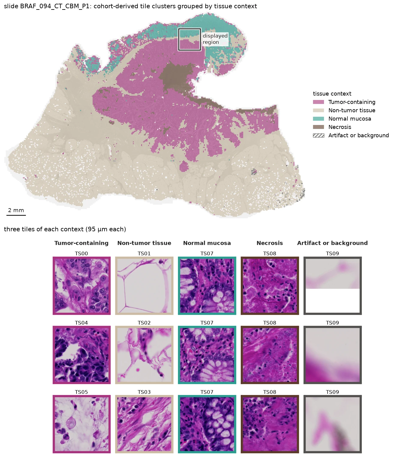
Cohort-derived tissue contexts on BRAF_094_CT_CBM_P1. The outlined region corresponds to the region enlarged in the overview figure. Example tiles were selected near their cluster centroids to show the morphology associated with each tissue context. Image from S-BIAD1407, CC BY 4.0.

Connect tissue context to cell annotations¶

Every encoded cell keeps the index of the tissue tile from which it was generated. The cohort-derived tissue context can therefore be attached directly to each cell.

for slide_id, cell_table in cell_tables.items():
    tile_cluster = (
        tile_tables[slide_id]
        .obs
        .set_index("alhena_tile_index")["tile_cluster"]
    )
    cell_table.obs["tile_cluster"] = (
        cell_table.obs["alhena_tile_index"].map(tile_cluster)
    )
    cell_table.obs["compartment"] = cell_table.obs[
        "alhena_celltype_compartment_v1"
    ].where(cell_table.obs["alhena_valid_compartment_v1"])

EXAMPLE_SLIDE = "BRAF/094_CT_CBM_P1"

cell_tables[EXAMPLE_SLIDE].obs[
    ["compartment", "tile_cluster"]
].head()

	compartment	tile_cluster
BRAF/094_CT_CBM_P1::0	Immune	TS03
BRAF/094_CT_CBM_P1::1	Immune	TS07
BRAF/094_CT_CBM_P1::2	Epithelial_Melanocyte	TS07
BRAF/094_CT_CBM_P1::3	Immune	TS03
BRAF/094_CT_CBM_P1::4	Immune	TS03

Cell-level annotations and tissue-level context can now be used together.

Because the nuclei and ALHENA tables share the same SpatialData coordinate system, both scales can be inspected in the same field.

EXAMPLE_FIELD_MIN = [87087, 9867]
EXAMPLE_FIELD_MAX = [93093, 15873]

example_sdata = sdatas[EXAMPLE_SLIDE]

field = sd.bounding_box_query(
    example_sdata,
    axes=("x", "y"),
    min_coordinate=EXAMPLE_FIELD_MIN,
    max_coordinate=EXAMPLE_FIELD_MAX,
    target_coordinate_system="global",
    filter_table=True,
)

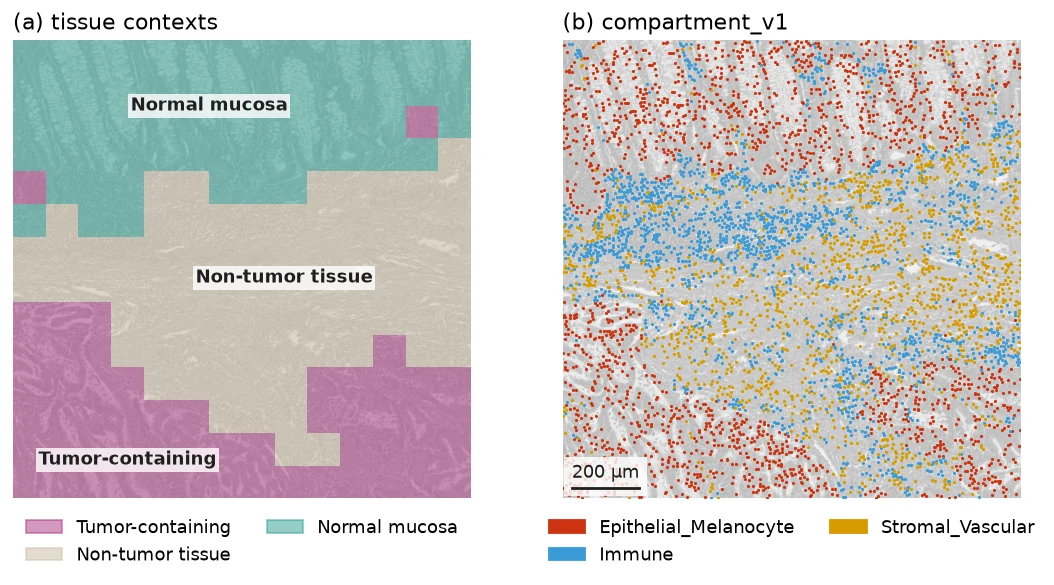
The same field shown with cohort-derived tissue contexts and ALHENA compartment_v1 annotations. Both are queried from the same SpatialData coordinate system. Image from S-BIAD1407, CC BY 4.0.

Query tumor-immune neighborhoods with Squidpy¶

Tissue context, cell annotation and coordinates can now be combined in one spatial question. Which Immune cells lie within the neighborhood of epithelial cells in tumor-containing tissue?

The neighborhood radius is set to approximately 44.65 µm, matching the distance threshold used in the published study.

SCALE = 2.009  # slide pixels per pixel of the published nucleus coordinates
NEIGHBORHOOD_RADIUS_PX = np.nextafter(100 * SCALE, 0.0)  # 100 published pixels, about 44.65 µm

TUMOR_CLUSTERS = ["TS00", "TS04", "TS05"]  # tumor-containing tissue contexts
NON_COUNTED_CLUSTERS = ["TS07", "TS08", "TS09"]  # normal mucosa, necrosis, artifact or background

epithelial_anchors counts the valid epithelial annotations on tumor-containing tiles. nearby_immune counts the valid Immune annotations within 44.65 µm of at least one of those anchors. Immune cells in normal mucosa, necrosis or artifact/background are not included in the neighborhood count.

rows = []

for slide_id, cell_table in cell_tables.items():
    obs = cell_table.obs
    tumor = obs["tile_cluster"].isin(TUMOR_CLUSTERS)
    non_counted_tissue = obs["tile_cluster"].isin(NON_COUNTED_CLUSTERS)

    obs["anchor"] = obs["compartment"].eq("Epithelial_Melanocyte") & tumor
    obs["eligible_immune"] = obs["compartment"].eq("Immune") & ~non_counted_tissue

    sq.gr.spatial_neighbors_radius(
        cell_table, radius=NEIGHBORHOOD_RADIUS_PX, key_added="neighborhood"
    )
    graph = cell_table.obsp["neighborhood_connectivities"]
    obs["near_anchor"] = (
        np.asarray(graph[:, obs["anchor"].to_numpy()].sum(axis=1)).ravel() > 0
    )
    obs["counted"] = obs["eligible_immune"] & obs["near_anchor"]

    rows.append(
        {
            "slide_id": slide_id,
            "patient_id": slide_manifest.loc[slide_id, "patient_id"],
            "nearby_immune": int(obs["counted"].sum()),
            "epithelial_anchors": int(obs["anchor"].sum()),
        }
    )

per_slide = pd.DataFrame(rows)

per_slide.head()

	slide_id	patient_id	nearby_immune	epithelial_anchors
0	BRAF/004_AT_PD_P1	BRAF-004	16947	117166
1	BRAF/006_AA_CBM_P1	BRAF-006	84	271
2	BRAF/008_AN_PD_P1	BRAF-008	33497	919060
3	BRAF/009_AS_PD_P1	BRAF-009	19629	298283
4	BRAF/010_AM_PD_P1	BRAF-010	66768	195162

The figure below reads these cell-level flags in a 0.5 mm crop of the example slide.

NEIGHBORHOOD_CROP = (86009, 11468, 2250)  # x, y, side in full-slide pixels

x0, y0, side = NEIGHBORHOOD_CROP

neighborhood_view = sd.bounding_box_query(
    sdatas[EXAMPLE_SLIDE],
    axes=("x", "y"),
    min_coordinate=[x0, y0],
    max_coordinate=[x0 + side, y0 + side],
    target_coordinate_system="global",
    filter_table=True,
)

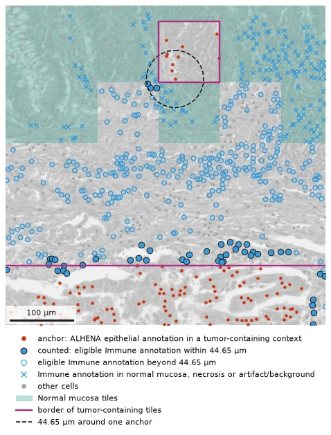
Example crop showing epithelial anchors and Immune cells classified by the spatial query above. Filled blue points are counted in nearby_immune. Open blue points are eligible Immune cells outside the 44.65 µm neighborhood. Crosses mark Immune cells in normal mucosa, necrosis or artifact/background, which are not included in the neighborhood count. The dashed circle marks the 44.65 µm neighborhood of one anchor. Image from S-BIAD1407, CC BY 4.0.

Where ALHENA and the published labels disagree¶

The published cell labels have not been used by ALHENA in any of the analyses above. They are introduced here only to compare the ALHENA annotations with the annotations reported for these cohorts in the original publication.

published_labels[slide_id] holds the published table of a slide: one row per published nucleus, indexed by cell ID, with its class (published_class) and its position in the published pixels (x_pub, y_pub). The eight published classes are mapped to the three compartment_v1 cell types.

PUBLISHED_COMPARTMENT = {
    "cep": "Epithelial_Melanocyte",
    "nep": "Epithelial_Melanocyte",
    "lym": "Immune",
    "mac": "Immune",
    "neu": "Immune",
    "fib": "Stromal_Vascular",
    "end": "Stromal_Vascular",
    "myo": "Stromal_Vascular",
}

labeled_slides = [
    cell_table.obs[["compartment", "tile_cluster"]]
    .dropna(subset=["compartment"])  # valid annotations only
    .join(published_labels[slide_id], how="inner")
    for slide_id, cell_table in cell_tables.items()
]
labeled = pd.concat(labeled_slides)
agreement = labeled["published_class"].map(PUBLISHED_COMPARTMENT).eq(labeled["compartment"])
print(f"{agreement.mean():.1%} ({agreement.sum():,} of {len(agreement):,} nuclei)")

73.3% (68,572,514 of 93,518,091 nuclei)

Because the published labels are themselves inferred from H&E, the 73.3% value should be interpreted as agreement between two H&E-based annotation systems.

ALHENA cell embeddings include information from the surrounding tissue. The next comparison asks whether agreement with the published labels changes as a published lymphocyte is surrounded by increasing numbers of published cancer epithelial cells.

from scipy.spatial import cKDTree


def crowding(labeled):
    """A slide's published lymphocytes, with the published cancer epithelial cells near each."""
    lymphocytes = labeled[labeled["published_class"] == "lym"]
    cancer_epithelial = labeled.loc[labeled["published_class"] == "cep", ["x_pub", "y_pub"]]
    n_cep = cKDTree(cancer_epithelial).query_ball_point(
        lymphocytes[["x_pub", "y_pub"]], r=np.nextafter(100.0, 0.0), return_length=True
    )  # strictly within 100 published pixels, about 44.65 µm
    return lymphocytes.assign(n_cep=n_cep)


lymphocytes = pd.concat([crowding(labeled) for labeled in labeled_slides])
bins = pd.cut(lymphocytes["n_cep"], [-1, 0, 2, 5, 10, 20, np.inf],
              labels=["0", "1–2", "3–5", "6–10", "11–20", ">20"])
in_tumor = lymphocytes["tile_cluster"].isin(TUMOR_CLUSTERS)
share_immune = lymphocytes["compartment"].eq("Immune").groupby([in_tumor, bins]).mean()

Share of published lymphocytes that ALHENA annotates Immune, by the number of published cancer epithelial cells within 44.65 µm, inside and outside tumor-containing tissue, across the cohort.

Outside tumor-containing tissue, agreement remains around 81 to 86%. Within tumor-containing tissue, agreement decreases as the number of nearby published cancer epithelial cells increases, from 70.8% with none nearby to 27.8% with more than 20.

The quantitative result shows where disagreement is most frequent. The images below let the reader inspect what those regions look like.

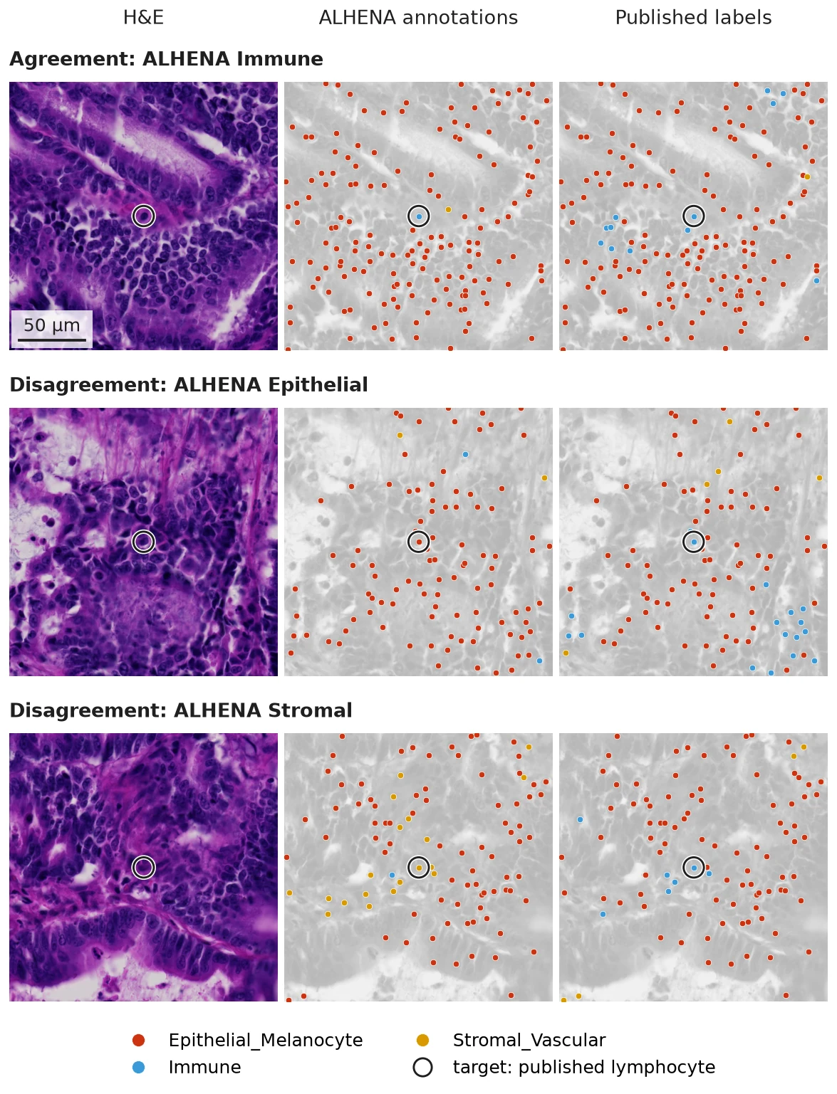
Three 200 µm fields centered on published lymphocytes with more than 20 published cancer epithelial cells within 44.65 µm in tumor-containing tissue. Each row shows the same field as H&E alone, with ALHENA compartment_v1 annotations, and with the published labels mapped to the same broad cell type classes. The target nucleus is marked in every panel. Image from S-BIAD1407, CC BY 4.0; published labels from Mendeley Data 9z48yfzr63, CC BY 4.0.

These examples show that disagreements can arise in morphologically complex tumor regions, where nuclei labeled as lymphocytes in the published annotations can lie among many nearby epithelial cells.

From slides to patients¶

So far, the analysis has stayed at tile and cell level. To move to the patient level, outputs from all available slides belonging to the same patient are pooled and summarized. This produces one feature vector per patient rather than one observation per tile or cell.

When a patient has multiple slides, counts are summed across slides before proportions, ratios or densities are calculated; slide-level values are not averaged. Spatial relationships, such as tile adjacency or cell neighborhoods, are first evaluated within each slide and their counts are then combined across the patient.

Tissue composition¶

A simple patient-level summary is tissue composition. For each patient, we pool all tissue tiles from all available slides and count how many belong to each tile cluster. TS09 (artifact or background) is left out, so tissue refers here to TS00–TS08.

The resulting features describe both the overall abundance of individual tile clusters and their composition within broader groups. For example:

• share_TS04 is the number of TS04 tiles divided by all tissue tiles from the patient.
• share_tumor is the number of tiles in the tumor-containing clusters TS00, TS04 and TS05 divided by all tissue tiles.
• share_non_tumor is the corresponding fraction for TS01, TS02, TS03 and TS06.
• TS04_in_tumor is the number of TS04 tiles divided by all tumor-containing tiles.
• TS02_in_non_tumor is the number of TS02 tiles divided by all non-tumor tissue tiles.
• necrosis_to_tumor is the number of TS08 tiles divided by the number of tumor-containing tiles.
• non_tumor_to_tumor is the number of non-tumor tissue tiles divided by the number of tumor-containing tiles.

These definitions produce 18 proportions and two ratios. Unlike the proportions, the two ratios can exceed 1 when the numerator contains more tiles than the denominator.

for slide_id, tiles in tile_tables.items():
    tiles.obs["patient_id"] = slide_manifest.loc[slide_id, "patient_id"]

cohort_tiles = pd.concat([tiles.obs for tiles in tile_tables.values()], ignore_index=True)
tissue = cohort_tiles[cohort_tiles["tile_cluster"] != "TS09"]  # artifact or background left out
per_cluster = pd.crosstab(tissue["patient_id"], tissue["tile_cluster"])  # tiles per patient

NON_TUMOR_CLUSTERS = ["TS01", "TS02", "TS03", "TS06"]
n_tissue = per_cluster.sum(axis=1)
n_tumor = per_cluster[TUMOR_CLUSTERS].sum(axis=1)
n_non_tumor = per_cluster[NON_TUMOR_CLUSTERS].sum(axis=1)

tissue_composition = pd.concat(
    [
        per_cluster.div(n_tissue, axis=0).add_prefix("share_"),
        (n_tumor / n_tissue).rename("share_tumor"),
        (n_non_tumor / n_tissue).rename("share_non_tumor"),
        per_cluster[TUMOR_CLUSTERS].div(n_tumor, axis=0).add_suffix("_in_tumor"),
        (per_cluster["TS08"] / n_tumor).rename("necrosis_to_tumor"),
        per_cluster[NON_TUMOR_CLUSTERS].div(n_non_tumor, axis=0).add_suffix("_in_non_tumor"),
        (n_non_tumor / n_tumor).rename("non_tumor_to_tumor"),
    ],
    axis=1,
)

tissue_composition.head().round(3)

	share_TS00	share_TS01	share_TS02	share_TS03	share_TS04	share_TS05	share_TS06	share_TS07	share_TS08	share_tumor	share_non_tumor	TS00_in_tumor	TS04_in_tumor	TS05_in_tumor	necrosis_to_tumor	TS01_in_non_tumor	TS02_in_non_tumor	TS03_in_non_tumor	TS06_in_non_tumor	non_tumor_to_tumor
patient_id
BRAF-004	0.293	0.006	0.157	0.076	0.023	0.071	0.153	0.199	0.021	0.386	0.394	0.758	0.059	0.183	0.054	0.016	0.400	0.194	0.390	1.020
BRAF-006	0.000	0.373	0.387	0.019	0.004	0.000	0.192	0.002	0.023	0.004	0.971	0.031	0.938	0.031	5.266	0.384	0.398	0.020	0.198	221.604
BRAF-008	0.700	0.038	0.024	0.169	0.013	0.045	0.002	0.000	0.008	0.758	0.234	0.923	0.018	0.059	0.010	0.164	0.104	0.721	0.011	0.309
BRAF-009	0.144	0.096	0.264	0.418	0.019	0.000	0.033	0.000	0.024	0.163	0.812	0.882	0.117	0.001	0.148	0.119	0.326	0.515	0.041	4.976
BRAF-010	0.294	0.047	0.244	0.259	0.018	0.000	0.037	0.011	0.090	0.312	0.587	0.942	0.057	0.001	0.288	0.080	0.416	0.442	0.063	1.880

Each row now represents one patient rather than one tile or slide.

Other patient-level summaries¶

Tissue composition is only one way to aggregate the stored ALHENA outputs. For the downstream analysis below, we construct six complementary patient-level feature blocks that retain different aspects of tissue composition, tissue organization, cell phenotypes, spatial organization or the learned tile representations.

Feature block	What is summarized for each patient	Features
Tissue composition	Relative abundance of individual tile clusters, composition within the tumor-containing and non-tumor groups, and ratios between selected tissue contexts	20
Tissue architecture	Shape and organization of tumor-containing tissue, together with adjacency patterns between tile clusters	28
Cell composition by tissue context	ALHENA epithelial, Immune and stromal cell composition and density across tissue regions, together with Immune heterogeneity within tumor-containing tissue	66
Cell spatial features	Local relationships between ALHENA-annotated cell types, including nearest-cell distances, neighborhood composition and Immune aggregates	77
Tile codebook	Distribution of the patient's tissue tiles across 32 clusters in ALHENA tile-embedding space	32
Mean tumor-tile embedding	Mean 1536-dimensional ALHENA tile embedding across the patient's tumor-containing tiles	1536

The 28 tissue-architecture features use the tile-cluster assignment and grid position of each tile. Seven features describe properties of the tumor-containing regions, including their edge fraction, depth, fragmentation and contact with surrounding tissue or necrosis. The other 21 measure whether selected pairs of tile clusters are adjacent more or less often than expected from their abundance.

The 66 cell-composition features summarize ALHENA epithelial, Immune and stromal annotations across 13 tissue regions, including tumor-containing tissue, individual tumor clusters, tumor edge and core, and non-tumor regions at increasing distances from tumor. They include cell-type fractions, total and Immune cell densities, and measures of how unevenly Immune cells are distributed across tumor-containing tiles.

The 77 cell-spatial features use the coordinates and ALHENA cell type of each cell to describe local cellular organization. They summarize, across several tissue regions, how often Immune cells lie close to epithelial or stromal cells, how cell types are represented among the ten nearest neighbors of each cell, and whether epithelial cells occur in isolated or stromal-rich neighborhoods. Additional features describe Immune-cell aggregates and their relationship to tumor-containing tissue.

The tile codebook provides a compact summary of the ALHENA tile embeddings without averaging them into a single vector. The tile-embedding space is first reduced by PCA and then divided into 32 clusters using k-means; the 32 cluster centers together form the codebook. Each tissue tile is assigned to its nearest cluster. For each patient, we calculate the fraction of tissue tiles assigned to each of the 32 clusters. These 32 values sum to 1 and describe how the patient's tissue is distributed across recurring patterns in ALHENA embedding space.

At the other end of the representation spectrum, the mean tumor-tile embedding retains ALHENA's full 1536-dimensional representation. For each patient, tile embeddings are averaged across all tiles belonging to the tumor-containing clusters TS00, TS04 and TS05.

sums = {}
counts = {}

for tiles in tile_tables.values():
    patient = tiles.obs["patient_id"].iloc[0]
    tumor = tiles[tiles.obs["tile_cluster"].isin(TUMOR_CLUSTERS)]

    sums[patient] = sums.get(patient, 0) + tumor.obsm["X_alhena_tile"].sum(axis=0)
    counts[patient] = counts.get(patient, 0) + tumor.n_obs

mean_tumor_tile_embedding = pd.DataFrame({
    patient: sums[patient] / counts[patient]
    for patient in sums
}).T

Together, these summaries form a patient-level feature library that can be reused for downstream analyses.

The patient-level feature library contains 165 patients from the published study with pretreatment primary-tumor slides available for these analyses.

MSI classification from patient-level features¶

The patient-level summaries can then be used to address downstream biological or clinical questions. As one example, we test how much information about MSI status is captured by each feature block.

MSI status is not an output predicted directly by ALHENA. Instead, we use the patient-level features derived from ALHENA outputs to train separate logistic-regression classifiers for MSI status.

MSI classification is evaluated in the 114 BRAF patients, including 35 microsatellite instability-high (MSI-H) and 79 microsatellite-stable (MSS) tumors. MISSONI is not used for this classification because all MISSONI patients in this dataset are MSI-H.

The patient-level feature library is prepared once, before cross-validation and without using MSI status. This includes the cohort-level feature definitions described above, median imputation of missing values and rank-based normalization where applicable. Imputation and normalization are performed separately within each cohort, and none of these steps is re-estimated within the cross-validation folds.

Classification is then evaluated with repeated nested cross-validation. Within each outer training fold, features are centered and scaled, feature blocks with more than 60 dimensions are reduced to 60 principal components, the L2 regularization strength is selected by inner cross-validation, and the logistic-regression model is fitted. The fitted transformations and classifier are then applied to the held-out patients.

AUC with its 95% confidence interval for each feature block, from repeated nested cross-validation in the BRAF cohort (114 patients, 35 MSI-H). The intervals resample patients within MSI status over the fixed out-of-fold predictions.

Tissue composition alone is close to chance. Tissue architecture, cell-level summaries and representation-level features carry more MSI signal in this cohort, with the mean tumor-tile embedding giving the highest AUC.

These downstream classifiers are trained and cross-validated within BRAF. Transfer to an independent cohort containing both MSI-H and MSS tumors is not tested.

Take-home¶

• Encode once. ALHENA produces tile and cell representations and cell annotations that can be reused across tissue, cell and spatial analyses without repeatedly encoding the H&E image.
• Stay in the scverse ecosystem. ALHENA outputs fit naturally into AnnData and SpatialData and can be combined directly with tools such as Scanpy and Squidpy.
• Move across scales and identify challenging contexts. The same outputs support tissue-context analysis, spatial cell queries and patient-level features. Comparison with the published annotations highlights contexts in which agreement is lower, particularly in tumor-containing tissue around published lymphocytes with many nearby published cancer epithelial cells.

Data and attribution¶

• Images: BioImage Archive S-BIAD1407, doi:10.6019/S-BIAD1407, CC BY 4.0.
• Nucleus positions and classes: Mendeley Data 9z48yfzr63, doi:10.17632/9z48yfzr63.1, CC BY 4.0.
• MSI status and the 44.65 µm proximity threshold: Trahearn N, et al. Computational pathology applied to clinical colorectal cancer cohorts identifies immune and endothelial cell spatial patterns predictive of outcome. J Pathol 2025;265:198–210. doi:10.1002/path.6378, CC BY 4.0.

H&E images shown on this page are cropped, downsampled, converted to grayscale or overlaid versions of the source images.

---

Next: How ALHENA works